Thursday 17 November 2011

Your Favourite Map Projection

...and what it says about you.


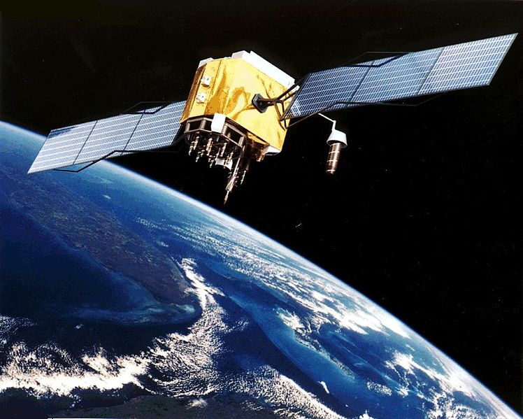
XKCD goes geospatial!  (Happens to everything eventually...)


Thursday 10 November 2011

OpenGeo Interview

My name in lights once again.  If this keeps up I'm going to have to start asking for an outrageous rider...


Thursday 27 October 2011

Sobering thought

According to this interesting BBC page on population, the number of humans on Earth has more than doubled in my lifetime.


Anyone who has spent time trying to speed up an O(n^2) algorithm knows this can't be a good thing...

Tuesday 25 October 2011

Using a web service for Elevation from JEQL

MapQuest has a whole range of useful and freely available web services for geospatial queries.  One of these is the Open Elevation Service.  I thought it would be interesting to try it out using JEQL's capabilities of querying URLs and plotting datasets as images.

The Open Elevation Service is extremely simple to use.  You just submit a URL containing the location:

http://open.mapquestapi.com/elevation/v1/getElevationProfile?callback=foo&shapeFormat=raw&latLngCollection=39.740112,-104.984856

and you get back a JSON (or XML) response with the elevation:

 foo({
"shapePoints":[39.740112,-104.984856],
"elevationProfile":[{"distance":0,"height":1616}],
"info":{"copyright":{"text":"© 2011 MapQuest, Inc.","imageUrl":"http://tile21.mqcdn.com/res/mqlogo.gif","imageAltText":"© 2011 MapQuest, Inc."},
"statuscode":0,
"messages":[]}
});

JEQL doesn't (yet) do JSON parsing, but it's easy to pick out the height attribute with a simple RegEx:

height = RegEx.extract(elevJson, \'"height":(-?\d+)\}');

Querying over a grid of locations provides a dataset which is a gridded Digital Elevation Model (DEM).  JEQL provides a function to generate a table which is a grid of integers, so it's easy to produce a grid of lat/long locations:

loc = select baseLat + i * cellSize lat, baseLon + j * cellSize lon
    from Generate.grid(1, gridSize, 1, gridSize);


Once the elevations for all locations are retrieved,  the locations are used to compute square cells (polygons) which cover the area, and the cells are symbolized with a fill value from a suitable color map based on elevation.

Here's the final result.  It's slightly squashed in aspect ratio, since the data grid is in the lat/long coordinate system.  The obvious data dropouts seem to be hard errors in the MapQuest service, which is slightly surprising.  But's it's recognizably Mt. St. Helens - you can even see the lava dome in the crater!


Not surprisingly, this isn't quick to generate - the service runs at about 10 queries per second.  (Actually, that seems pretty reasonable for a free web service!).  The service does support querying multiple points per request - I might try to see if this decreases the latency (although this might be a bit complex to express in JEQL).

Here's the whole script:

//--------------------------------------
//
// Plots a DEM generated using the MapQuest Elevation service
//
//--------------------------------------
baseLat = 46.16 ;  baseLon = -122.25;    // Mt St Helens
areaSize = 0.10;
gridSize = 100;
cellSize = areaSize / gridSize;

//---- Generate location grid
loc = select     baseLat + i * cellSize lat,
        baseLon + j * cellSize lon
    from Generate.grid(1, gridSize, 1, gridSize);

//---- Query elevation service for each grid point
telev = select lat, lon, elevJson, elev
    with {
        url = $"http://open.mapquestapi.com/elevation/v1/getElevationProfile?callback=foo&shapeFormat=raw&latLngCollection=${lat},${lon}";
        elevJson = Net.readURLnoEOL(url);
        height = RegEx.extract(elevJson, \'"height":(-?\d+)\}');
        elev = Val.toInt(height);
    }
    from loc;
Mem telev;

//---- Create raster cell boxes, symbolize with color map based on elevation, and plot
minElev = 800.0; maxElev = 2500.0;
tplot = select Geom.createBoxExtent(lon, lat, cellSize, cellSize) cell,
        Color.interpolate("00a000", "ffb000", "aaaaaa", "ffffff", index) style_fillColor
    with {
        index = (elev - minElev) / (maxElev - minElev);
    }
    from telev;

textent = select geomExtent(cell) from tplot;

Plot     extent: val(textent)
    data: tplot
    file: "dem.png";

Monday 24 October 2011

(r-i-p (john mccarthy))

John McCarthy, inventor of LISP, has died at age 84. 

Having finally balanced his parentheses, his atoms can now be returned to the free list.

Jobs, Ritchie, McCarthy - so many of the greats passing....


Friday 7 October 2011

Extracting GTFS data using JEQL

Once you understand the General Transit Feed Specification (GTFS) data model, the next step is to transform the data into a format usable in GIS tools.  As usual, that means shapefiles (sigh...).  Here's a JEQL script that extracts the geometry of all unique trips (aka "route patterns"), as well as the stop locations.

Some interesting aspects of the script:
  • the GTFS spatial data is in geographic coordinates (lat/long). The script projects this into BC-Albers (EPGS code 3005) using the CRS.project() function.  Many other coordinate systems could be used (or none - e.g. for output to KML)
  • the geomConnect()aggregate function connects Points into LineStrings


/*=======================================================
Extracts Trips (with shapes) and stops from from a GTFS dataset. 
Includes shape, trip and route information.
Spatial data is converted from Geographic to BC-ALbers

Usage Notes:
- indir: directory containing the input GTFS files
========================================================*/

indir = "";  outdir = "";

//========================================================
//  Extract Trips with unique linework, with route information
//========================================================
CSVReader tshape hasColNames: file: indir+"shapes.txt";
CSVReader ttrip hasColNames: file: indir+"trips.txt";
CSVReader troutes hasColNames: file: indir+"routes.txt";  
Mem troutes;

crs_BCAlbers = "EPSG:3005";

//--- extract unique shapes
trips = select distinct route_id, trip_headsign, shape_id 
    from ttrip;

//--- extract trip pts and order them in sequence
tpt = select shape_id, Val.toInt(shape_pt_sequence) seq,
		Geom.createPoint(Val.toDouble(shape_pt_lon), 
                                 Val.toDouble(shape_pt_lat) ) pt
	from tshape
	order by shape_id, seq;

//--- connect pts into lines and project
tline = select shape_id, 
     CRS.project(Geom.toMulti(geomConnect(pt)), crs_BCAlbers) geom
	from tpt
	group by shape_id;
	
//--- join route info to trip shape
trouteLines = select r.route_id, r.agency_id, 
    r.route_short_name, r.route_long_name,
    r.route_type, r.route_url,
    trip_headsign, l.*
        from tline l
        join trips t on t.shape_id == l.shape_id
        join troutes r on r.route_id == t.route_id;

ShapefileWriter trouteLines file: outdir+"gtfs_trips.shp";

//========================================================
//  Extract Stop points
//========================================================
CSVReader tstopsRaw hasColNames: file: indir+"stops.txt";

tstop = select stop_id,stop_code,stop_name,stop_desc,
        CRS.project(Geom.createPoint(
	    Val.toDouble(stop_lon), 
	    Val.toDouble(stop_lat) ), crs_BCAlbers) pt,
        zone_id
        from tstopsRaw;

ShapefileWriter tstop file: outdir+"gtfs_stops.shp";

Using this script on the GTFS data for Metro Vancouver (available from TransLink here) produces a dataset that looks like this:


JTS & GEOS Wordles

For my JTS talk at FOSS4G I created a couple of Wordles showing systems which use JTS and GEOS.  Here they are for posterity (and because I love seeing Wordles...)


Thursday 29 September 2011

Lars Rasmussen on the startup of Google Maps

Here's some interesting background to where Google Maps came from.  Must feel pretty good to have created a revolution (slippy maps) - and maybe to have just missed creating another one (Google Wave as an alternative to email).


Tuesday 27 September 2011

Data model diagrams for GTFS

Recently I've been doing some work with the General Transit Feed Specification (GTFS).  This is a simple data model initiated by Google, in order to allow transit organizations to publish their schedules for routing and visualization purposes.

As usual, Google has nice, succinct documentation for the GTFS format (which is a set of CSV files embodying an implicit data model).  But I was surprised to find that they don't provide any kind of data model diagram showing the relationships between the various entities (files) in the model.  I have a feeling that they think this would be "too technical" for users - or maybe they just don't believe in using a long-established body of theory?

So, to help my understanding of GTFS I put together a simple diagram of the data model.  I used Google Diagrams, which is why this looks a little primitive.   (Hmmm... maybe another reason they don't do diagrams is that they are religious about dog-fooding?)


After doing this I found the paper A Transmodel based XML schema for the Google Transit Feed Specification, which has a much more detailed UML model of GTFS:


The end goal of doing all this was to be able to transform a GTFS data feed into shapefile format.  For this I used a simple JEQL script.  But that's another blog post.

Monday 19 September 2011

Paul Ramsey's Keynote at FOSS4G 2011

As usual, Paul delivered a highly amusing and thought-provoking keynote at FOSS4G 2011.  For the benefit of the hard-core twitterless, the slides are here.


Thursday 1 September 2011

Everything you wanted to know about UK Coordinate Systems

Those helpful folks at the UK Ordnance Survey have provided a fine reference Guide to Coordinate Systems in Great Britain.  It's well worth reading if you're interested in the intricacies of coordinate systems, datums, surveying and GPS.  It's a bit technical, but if you can handle coding in Javascript you can probably get something out of it...

An interesting extract gives the general flavour:
  • The WGS84 Cartesian axes and ellipsoid are geocentric; that is, their origin is the centre of mass of the whole Earth including oceans and atmosphere.
  • The scale of the axes is that of the local Earth frame, in the sense of the relativistic theory of gravitation.
  • Their orientation (that is, the directions of the axes, and hence the orientation of the ellipsoid equator and prime meridian of zero longitude) coincided with the equator and prime meridian of the Bureau Internationale de l’Heure at the moment in time 1984.0 (that is, midnight on New Year’s Eve 1983).
  • Since 1984.0, the orientation of the axes and ellipsoid has changed such that the average motion of the crustal plates relative to the ellipsoid is zero. This ensures that the Z-axis of the WGS84 datum coincides with the International Reference Pole, and that the prime meridian of the ellipsoid (that is, the plane containing the Z and X Cartesian axes) coincides with the International Reference Meridian.
  • The shape and size of the WGS84 biaxial ellipsoid is defined by the semi-major axis length a  6378137.0 metres, and the reciprocal of flattening 1/f  298.257223563. This ellipsoid is the same shape and size as the GRS80 ellipsoid.
  • Conventional values are also adopted for the standard angular velocity of the Earth, and for the Earth gravitational constant. The first is needed for time measurement, and the second to define the scale of the system in a relativistic sense.
Now then, if you find yourself getting lost on the way from Foyle's to the nearest Lyon's tea shop, you can't say you haven't been warned!


Wednesday 24 August 2011

Interview with Directions Magazine

The Twittersphere is buzzing with my latest (well, only) interview with Directions Magazine on the State of the JTS Topology Suite.


Props to Rob Rutherford and Amber Weber at Clover Point for setting this up!

Thursday 14 July 2011

Would you be lost without it?

Nowadays GPS is ubiquitous in electronic gadgets (no electric toothbrush is complete without it!) GPS is a classic example of iceberg technology 1. An output which in one sense verges on trivial - two numbers! - in fact relies on a huge unseen infrastructure of technology, physics, organizations, and yes, government funding.

The UK Telegraph has an interesting article on GPS 2 covering some of the technical, scientific, historic and political background to the system.


On a side note, I'm happy to observe that statements like this aren't as common as they used to be:

Slightly worryingly, when I was invited to watch a “contact” in another control room earlier in the day, the software crashed and a familiar, blue Microsoft Windows screen appeared on the wall


Notes:
  1. yes I made this up. My entry for Internet memedom!
  2. don't worry, it's still safe to use your cellphone after visiting this site

Sunday 26 June 2011

JTS 1.12 released

JTS 1.12 has been released, and is now available for download at SourceForge.

Some highlights of this release include:
... along with many other features, enhancements and fixes.


Single-Sided Buffer

Wednesday 8 June 2011

Apple walls getting higher

ZDNet has an interesting long view on the Apple iCloud announcement. Money quote:
The mobile world is moving away from the chock-full-o’-content web and increasingly becoming a world of closed pipes of content, with Apple, Google, HP and Microsoft regulating the flow. Tech fiefdoms scattered across a vast open land have expanded into warring nation-states with adjacent borders. The Mac vs. PC vs. Linux argument from the early days of consumer computing has lost a great deal of its luster in recent years with the development of cloud computing on the open web, but the concept of platform wars is quickly making up for lost ground with the development of cloud computing in the closed mobile space.
I've always found the Apple walled garden a bit scary in its restrictions. Now the walls are getting higher and thicker - and other vendors will be following suit as fast as they dare.

I don't find Google's garden as threatening, for some reason. Perhaps because they have a different business model, based on page views rather than selling devices or software. For now that encourages them to not put any limits on where and how you access their services. But will that change if the Chromebook takes off? Is the fact that Honeycomb is not open source a tiny black cloud on the horizon?


Monday 6 June 2011

Java gets Reheated at OSCON

It's good to see that O'Reilly is adding a Java flavour to the OSCON conference. They have a good blog post highlighting why they think Java (and the JVM) is still one of the most important programming platforms around, especially for open source development.


Some of the interesting Java projects that will be covered at the conference are:
  • Incanter, a Clojure-based statistics library (this project is particularly interesting to me, since it overlaps with some of the target space of JEQL)
  • Gradle, a Groovy DSL for building, testing, and deploying software
  • Jenkins, a continuous integration platform
  • Neo4J, a graph database
Some may think that Java is entering the Red Giant phase of language evolution, but it still has the capacity to throw off some powerful solar flares. The longer the coffee pot sits on the stove, the stronger it gets...

Thursday 19 May 2011

JTS arrives in JavaScript

As I predicted back in 2008, JTS has now colonized the JavaScript ecosystem, thanks to the work of Bjorn Hartell on JSTS. At least, the project has been launched - it's a bit unclear as to how much functionality is actually there.

I hope to see some slick browser-based UI clients pop up, using Canvas or perhaps SVG?

The language scorecard for JTS now looks like:

[Update: Jan 31 2013] - Added R to the list

Wednesday 4 May 2011

FOSS4G is the place to be!

FOSS4G 2011 is happening in Denver this September.


I've submitted two abstracts for presentations:


Spatial Processing using JEQL

JEQL is a simple yet powerful language designed for expressing spatial (and non-spatial) processes. It follows the Table-Oriented Programming paradigm and provides a SQL-like query language. This talk gives an overview of JEQL and show some examples of its use.


What's New in JTS

The JTS Topology Suite has had numerous improvements in the past few versions. These include performance improvements, bug fixes and new functionality such as Delaunay Triangulation, Single-Sided Buffers, and Hausdorff Distance. This talk will discuss the new features, and demonstrate them using the JTS TestBuilder utility. Potential further features will be presented for discussion.


Vote early, vote often - and vote for me!

See you in Denver....


Friday 8 April 2011

Polygon Triangulation via Ear-Clipping with Delaunay Refinement

After this thread on the JTS list Michael Bedward was inspired to create a polygon triangulation algorithm using the Ear-Clipping approach. Standard Ear-Clipping algorithms don't handle polygons with holes, but Michael made a nice extension to do this. (David Eberly has a good write-up on this subject here, and of course there's always Wikipedia). One problem with ear-clipping is that it produces sub-optimal triangulations (in the the sense that it creates lots of very skinny triangles, which are visually and computationally unappealing). I suggested that he add a refinement step based on "flipping triangles" to improve the quality of the output triangle mesh. This is similar to the approach used in Delaunay triangulation algorithms, and in fact it turns out that a good flipping criteria is to test for the Delaunay condition. (Two adjacent triangles which form a convex quadrilateral are Delaunay if neither lies in the circumcircle of the other. Wikipedia has a nice visual explanation). This code will get added to JTS in the next release. In the meantime, here's some cool pictures showing how it works. A gnarly test polygon:
Before refinement
After refinement
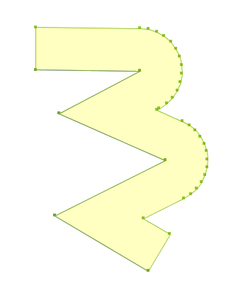
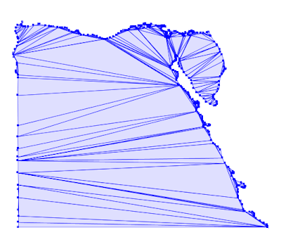
A country that has been in the news recently:
Before refinement
After refinement
Update (Nov 1, 2021): JTS now has Polygon Triangulation code.  See this post for details.

Dynamic Views in Google Blogs

Check out the cool new Dynamic Views feature for Google Blogs. I'm not sure how useful this is actually going to be for readers (especially since you have to do URL editing to invoke them - WTB!? (Where's The Button 8^)

But they sure look purty. Here's a shot of the Flipcard view:

Thursday 7 April 2011

Slope/Aspect/Elevation using JTS

David Skea is a longtime colleague, JTS contributor, and all-around geospatial guru. He's developing a Slope/Aspect/Elevation service to be used in forestry-related applications here in British Columbia. His work is a nice example of using JTS to perform real-world spatial processing.

The key to computing slope, aspect and elevation is to have a Digital Elevation Model (DEM) available for the terrain in the area of interest. In this case, the terrain data is provided by the TRIM irregular DEM, which is a dataset of over 500 million mass points covering all of British Columbia. To compute the required values for a given polygon, the first step is to extract only the mass points in the immediate region of the polygon (i.e. using the polygon envelope with a suitable buffer distance. The JTS Delaunay Triangulation API is used to compute a TIN triangulation from the TRIM mass points.


Using a JTS PointOnGeometryLocator, the triangles whose centroids lie in the polygon are selected. Since each mass point has an elevation value, each TIN triangle is located in 3D space. The normal vector can be computed for each triangle, which provides the slope and aspect values. The elevation is the height of the triangle centroid.

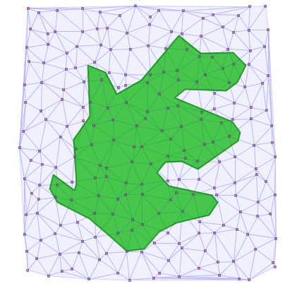
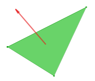
The SEA values for the triangles are averaged to compute the overall slope, aspect and elevation value for the polygon.

Here's a screenshot showing the results, using Google Earth as a convenient 3D visualization tool (click for full-size image).

Thursday 3 March 2011

GeoGeeks presentation on Geometry Libraries

Paul Ramsey has been doing his usual excellent work of promoting geo-geekery by setting up a Victoria GeoGeeks Meetup. Tonight I gave a presentation on Geometry Libraries for Fun and Profit.


I was intending to give it back-to-back with a presentation on JTS, to make the whole subject more concrete - but I rambled on for so long I was yanked from the stage before I could start on the second one! That's actually good, since it will give me time to polish up the presentation a bit more. In the meantime, the current slide deck is here: JTS - A Libary for Geometry Processing.

Tuesday 11 January 2011

Charting with JEQL

SQL has an elegant syntax for grouping and aggregating data. Java has powerful libraries for charting and graphing (like JFreeChart). JEQL has easy handling of tabular data. These go together like chocolate and peanut butter - and, um, more chocolate. Put them all together and you get this code:

CSVReader troute hasColNames: file: "routeLine2.csv";

tCityCount = select count(*) cnt, fromCity city
from troute
group by fromCity
order by cnt desc;

tdata = select city key, cnt value from tCityCount limit 20;

Chart type: "bar"
data: tdata
extrude:
color: "00c0f0"
showItemLabels:
xAxisTitle: "Top Cities by Originating Air Routes"
xAxisLabelRotation: -0.5
width: 1000
file: "cityRoutes.png";


producing this graph:


This uses the same air routes dataset created in a previous example, with a simple grouped summary to show the 20 cities with the most air routes originating in them.

JFreeChart is a bit notorious for being hard to use, but the JEQL command hides all the gory details behind a much simpler (but still powerful) Chart command interface. Currently Bar, XY, and Pie charts are supported. It will be easy to add other chart types as required.

Also on the ToDo list is to provide an option to emit Google Chart URLs, using the same set of options (at least, the ones that are applicable - and maybe some new ones).

Note: this is an experimental extension, which is not in a final state in the current JEQL release.

Thursday 6 January 2011

JEQL 0.9 released

Good news for those who wanted to try out the geodetic air routes JEQL script. The script requires JEQL version 0.9 to run. This version is now available for download.